.jpeg)
Two years ago Facebook announced a collaboration between their AI research department and the NYU Langone School of medicine and named the project fastMRI. Their goal? Make MRI acquisition significantly faster. A recent publication [1] stated that acquisition times could be accelerated 4 to 8 times using their deep learning approach on image reconstruction, without loss of image quality. Practically that would imply making a MRI scan of the knee in roughly 5 minutes, which is pretty fast. In this blog I will address two important questions: “How do they do it?” and “Is it safe?”
Assessment of abnormalities of anatomic structures is the basis of traditional radiology. In clinical practice a diagnostic image is evaluated for the presence of image features that differ from ‘normal’ with respect to the observer’s frame of reference. Simply put, the higher the image resolution (provided that signal-to-noise ratio remains the same) the easier it is for a radiologist to accurately assess these images.
Basically image quality can be seen as a function of the amount of information and noise obtained during the acquisition of that image. In general, more information can be acquired if more energy is used during acquisition. For MRI in practice, this means increasing either the strength of the magnetic field or the acquisition time can be uncomfortable for patients (and expensive as MRI-time is scarce in clinical practice).
Several algorithms have been developed to increase image resolution (actually, methods often aim to accelerate acquisition time while maintaining image quality), for example compressed sensing. Unsurprisingly, with the rise of artificial intelligence applications in medicine, deep learning to increase image quality has been a topic of several studies as well.[2]
One of my main concerns is: “are these methods safe?”. In essence these deep learning models are trained to find ‘additional image signal’ without putting in additional energy. But where does this signal come from? Will these models be able to reconstruct the anatomy of a patient or will they mimic general anatomic patterns of patients included in the training data (and thus potentially missing diagnoses)? To get to the bottom I will break down fastMRI’s recently published work to understand what happens within these algorithms.
Magnetic resonance imaging is a complex technique based on the magnetic properties of protons. I will not cover the inner workings of MRI, but basically during acquisition radio-frequent pulses are used to affect the alignment of the protons to the magnetic field. As the protons return to their equilibrium state energy is released, which is measured by receiver coils. These measurements are represented in the spatial frequency domain (called k-space). By applying a mathematical transformation (called inverse Fourier transform), this k-space can be converted into an MR image as we know it. For the sake of simplicity I will refer to k-space as raw (image) data.
In general, acquiring more raw data will increase image quality, but will increase acquisition time as well. As said before, shortening scanning time is both patient friendly and enables more patients to be scanned in the same amount of time (shortening waiting list and reducing the costs for an MRI scan). Prior to the deep learning era, two main methods were proposed for speeding up MRI scans: parallel imaging and compressed sensing. In parallel imaging multiple receiver coils (which are just devices that acquire signal during an MRI scan) are used after which the images are combined using sensitivity maps. Each coil only has to sample a part of the data, shortening the length of acquisition.
The second method, Compressed Sensing (CS), is an image reconstruction technique. It is based on the feature that images contain many pixels lacking unique information. For example photos can be reduced significantly in size using formats like jpeg. CS reasons the other way around: is it possible to reconstruct MR images with only sparsely sampled raw data and without loss of quality compared to if all raw data was sampled? CS can be seen as an optimization problem that can be solved by iterative gradient descent methods.[3] The main problem with reconstructing images with sparsely sampled raw data is that the reconstruction algorithm can not exactly establish from which position in the body a signal comes from. As a result, aliasing (or wrap-around) artifacts can be seen that project parts of the anatomy in wrong locations.
Recently deep learning has been used to optimize the CS approach. CS only works if the raw data is randomly sampled. However, due to the nature of the (most frequently) used sampling method in MRI (2D Cartesian sampling), fulfilling this can be complicated. Another challenge is the large amount of time necessary to reconstruct images. In addition, tuning hyperparameters (especially regularization) is challenging and have large consequences for the practicality of the images; over-regularization leads to smooth unnatural looking images, while under-regularized images still shows artifacts like aliasing.
Deep learning methods aim at these challenges: reconstruct images from under-sampled raw data without fulfilling the CS constraints and by dynamically learning the regularization parameters. The main difference between the deep learning and classical CS approaches is that in classical CS each image reconstruction is treated as a new optimization problem. The new deep learning approaches use information of i.e. the expected anatomy appearance and the known artifact patterns learned during training. The idea is that, during inference, under-sampled data can be reconstructed by the model, which is a lot faster than the classical approach.[4]
Variational Network
FastMRI builds upon the variational network (VarNet) as described by Hammernik et al. [4]. VarNet contains a shallow Convolutional Neural Network (CNN) of which the parameters are learned during a training process with iterative steps. VarNet uses multiple receiver coils and combines the information of all coils (based on sensitivity maps) in the reconstruction phase. However, for the sake of simplicity we ignore the multiple inputs and sensitivity maps.
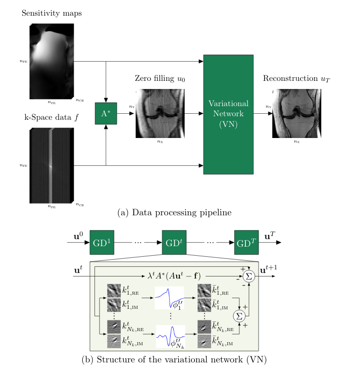
The input of the network is sparsely sampled raw data. During the first forward pass, all raw data that is not sampled is filled with zeros. This zero-filled data is transformed into an image. The image and sparsely sampled data are fed into the network.
In each step, the image is updated using two pathways (see Figure 1b). One pathway calculates the difference between the image of the previous forward pass (Fourier transformed into it’s raw data representation) and the original raw data input; any differences (multiplied by a weight λ specific for this forward pass) are subtracted from the image. In parallel the input image is mapped to an output image of the same shape by a shallow CNN with a non-linear activation function, which are summed and also subtracted from the input image. This results in a reconstructed output image, which is compared to a ground truth (MR image reconstructed in the normal way with fully sampled raw data) by assessing the mean squared error. Using gradient descent the kernels and non-linear activation functions of the CNN and the weights λ are updated. These steps are repeated a predefined (T) number of times.
fastMRI’s End-2-End-VarNet
The latest work from the fastMRI project describes a model that builds upon the original VarNet with several architectural adjustments and is named End-2-End-VarNet.[1] The model also uses multiple receiver coils and in contradiction to the original VarNet, uses a U-Net architecture to estimate sensitivity maps per receiver coil. Although I will skip this part, the result is that the calibration of the different receiver coils can be done much faster.
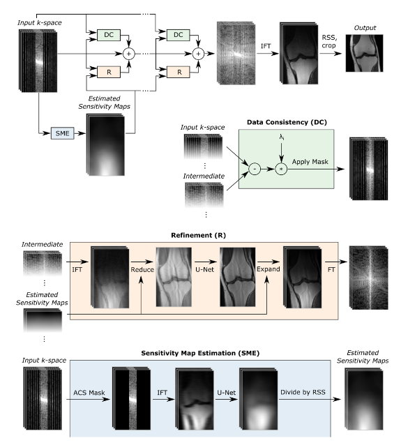
The other main architectural difference is the use of a U-net instead of a shallow CNN during each forward pass. Figure 2 depicts the algorithm’s architecture schematically. If we ignore the sensitivity map estimation, the steps are similar to the original VarNet. During each step in the training process, sparsely sampled raw data is passed forward into the network and updated by a data consistency (DC) and refinement (R) block. The DC-block compares the intermediate raw data (which is the output of the previous training step) with the original sparsely sampled raw input data and penalizes for any differences introduced during previous training steps multiplied by a factor λ. The R-block maps the input image into an image of the same size using an U-net architecture. The intermediate raw data is then combined with the output of the DC- and R-block. At the end of each training step the raw data is transformed into an MR-image which is compared to the ground-truth image by calculating the structural similarity loss. Gradient descent is used to update the parameters of the U-net and the factor λ.
The structural similarity loss function differs from the mean squared error (used in the original VarNet paper for optimization) in a sense it not does not only calculate the differences in individual pixels (which MSE does), but also takes into account perceived changes in structural information by comparing regions of the image and taking into account luminance, contrast and structure.[5] (Although not used for optimization, the original VarNet paper does report structural similarity loss in the result section).
The original VarNet was trained on MRI scans of 10 patients and tested on scans of 10 other patients. VarNet largely outperformed traditional CS methods (as implemented by multiple vendors) in case of MSE and structural similarity index measure (SSIM). The paper also presents some clear visual examples of the improvements regarding image quality and artifact reduction in the VarNet reconstructions compared to traditional CS methods. The most relevant finding was that the model was able to reconstruct high quality images of patients with pathology not present in the training data, which is of course essential when implemented in clinical practice.
The End-2-End-VarNet was able to outperform VarNet in case of SSIM.[1] However, while measuring error like SSIM is important, clinical studies are necessary to test the feasibility and safety of these algorithms in practice. My main concern is that, during inference, information of the training data is blended in with the current reconstructions; in this case image quality will be pretty good, although the image does not reflect the true anatomy of a patient. In addition, small abnormalities may be missed as these may be interpreted as noise by the model and polished away during inference. Luckily, researchers of the fastMRI project acknowledge this limitation and state that “quantitative measures only provide a rough estimate for the quality of the reconstructions and rigorous clinical validation needs to be performed before such methods can be used in clinical practice to ensure that there is no degradation in the quality of diagnosis.”.
Recently a clinical validation study was published [6] which claims no loss in diagnostic accuracy with a 3.5-fold acceleration (while sampling only 75% of raw data). This would translate to an MRI-acquisition time of roughly 5 minutes, which is quite impressive. The model was trained on 242 knee MRI exams, validation done on 56 MRI scans and the test set contained 108 MRI exams. The main result of the study was that agreement between different radiologists for the presence of several abnormalities was similar if both were shown the standard clinical images compared to the agreement if one of the radiologist was shown the accelerated images. The authors concluded that the imaging sequences thus are ‘interchangeable’. In addition, the subjective quality of the images reconstructed with deep learning was better, and only one out of six readers were able to correctly distinguish between the standard- and accelerated images.
Conclusion
I answered the questions how MRI acquisitions are speed up using deep learning and demonstrated promising (clinical) results from scientific literature. Now it is time to answer: are these algorithms safe and ready to use in clinical practice?. In my opinion, they aren’t (yet). The deep learning methods are promising and seem to learn mapping of artifact to non-artifacts and are penalized if the output derange from the original input raw data. However, as during training visual information of anatomical features is preserved in the U-net kernels, I am still not fully convinced, this information is not affecting the anatomical representation in MRI images. I do have to give credits to the fastMRI project for their transparancy. The full code can be found online on GitHub (https://github.com/facebookresearch/fastMRI) and researchers are invited to build upon the work of fastMRI and validate the algorithms in new (and larger) patient cohorts. The fastMRI research group “hopes that hardware vendors will get FDA approvals to bring these algorithms into production“ and I think that is the way to go.
Rik Kraan is a medical doctor with a PhD in Radiology working as a data scientist at Vantage AI, a data science consultancy company in the Netherlands. Get in touch via rik.kraan@vantage-ai.com
[1] Sriram, A, Zbontar J, Murrell T, et al. End-to-End Variational Networks for Accelerated MRI Reconstruction. arXiv2004.06688v2
[2] Harvey H, Topol EJ. More than meets the AI: refining image acquisition and resolution. The Lancet. 2020;396(10261):1479.
[3] David Donoho. Compressed sensing.IEEE Transactions on Information Theory, 52(4):1289–1306, 2006.
[4] Kerstin Hammernik, Teresa Klatzer, Erich Kobler, Michael P. Recht, Daniel K. Sodickson, Thomas Pock,and Florian Knoll. Learning a variational network for reconstruction of accelerated MRI data.MagneticResonance in Medicine, 79(6):3055–3071, 2018
[5] Image Quality Assessment: From Error Visibility to Structural SimilarityZhou Wang, Member, IEEE, Alan Conrad Bovik, Fellow, IEEE, Hamid Rahim Sheikh, Student Member, IEEE, andEero P. Simoncelli, Senior Member, IEEE
[6] Recht MP, Zbontar J, Sodickson DK, et al. Using deep learning to accelerate knee mri at 3 t: results of an interchangeability study. American Journal of Roentgenology. Published online October 14, 2020:1–9