
.jpeg)
A deep dive into the mathematical intuition of these frequently used algorithm.
Both classification and regression problems can be solved by many different algorithms. For a data scientist, it is essential to understand the pros and cons of these predictive algorithms to select a well-suited one for the encountered problem. In this blog, I will first dive into one of the most basic algorithms (a decision tree) to be able to explain the intuition behind more powerful tree-based algorithms that use techniques to counter the disadvantages of these simple decision trees. Tree-based algorithms have the advantage over linear or logistic regression in their ability to capture the nonlinear relationship that can be present in your data set. Compared to more complex algorithms such as (deep) neural networks, random forests and gradient boosting are easy to implement, have relatively few parameters to tune and are less expensive regarding computational resources and (in general) require less extensive datasets. The main goal of understanding these intuitions is that by grasping the intuition, using and optimizing the algorithms in practice will become easier and will eventually yield better performance.
Decision trees
A decision tree is a simple algorithm that essentially mimics a flowchart making them easy to interpret. A tree is composed out of the root-node, several tree-nodes and leaves. Essentially every node (including the root-node) splits the data set in subsets. Each split resembles an essential feature-specific question is a certain condition present or absent? Answering all those questions, until the bottom layer of the tree is reached, yields a prediction for the current sample. The leaves in this bottom layer are the last step in a decision tree and represent the predicted outcome.
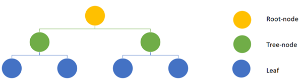
A schematic overview of a simple decision tree
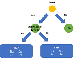
So far, so good: but now comes the interesting part. Let’s start with classification trees and imagine we have a sample data set with features regarding the presence of shortness of breath, coughing and fever and we want to predict if a patient has the flu. How can we figure out which feature should be the root-note and how our tree should be built to maximize the accuracy of the predictions?
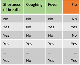 Note: This example will only use categorical features, however, one of the major advantages of trees is their flexibility regarding data types.
A decision tree is built from top to bottom using the training set, and at each level, the feature is selected that splits the training data best with respect to the target variable. To determine which feature splits the data set ‘best’, several metrics can be used. These metrics assess the homogeneity of the subsets that arise if a certain feature is selected in the node. The most often used metrics are ‘Gini impurity’ and ‘information gain entropy’. These metrics often yield a similar result [1] and since calculating Gini impurity does not include the use of a logarithm it might be slightly faster. The goal of calculating the Gini impurity is to measure how often a randomly chosen element from a set would be incorrectly labeled.
Let’s start at the root note: to select which features should be on top of the decision tree, first the Gini impurity for all individual features will be calculated.
The formula of the Gini impurity is
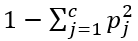
where c is the number of classes and Pj the fraction of items labeled with class j. As the prediction variables has 2 classes (Flu or no Flu) for each leaf the impurity is 1 — (P-no flu)² — (P-flu)².
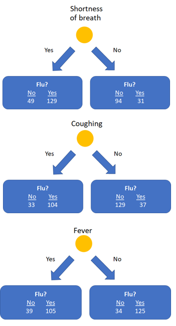
In our example (see the above image) the Gini impurityfor the left leaf of shortness of breath is: 1 - (49/(49+129))² - (129/(49+129))² = 0.399. The right leaf has an impurity of 1 - (94/(94+31))² - (31/(94+31))² = 0.372.
Finally, the final impurity for the root node shortness of breath can be calculate as the weighted average of the impurity of the two leaves: ((49+129)/(49+129+94+31)) * 0.399 + ((94+31)/(49+129+94+31)) * 0.372 = 0.388.
We can do this for the feature coughing and fever as well, which yield impurities of 0.365 and 0.364, respectively.
As fever has the lowest impurity, it is the best feature to predict if a patient has the flu and is therefore used as root node. After selecting fever as feature in the root node, the data is split up in two impure nodes with 144 samples on the left side and 159 samples on the right side.
Subsequently, we calculate the impurity for the other features shortness of breath and coughing for these created subsets to decide which feature should be used for the next node. Here the impurity for shortness of breath as next feature after the root node is 0.359. Let’s assume this impurity is less than coughing. The next step is to compare the impurity of the newly added node with the impurity of the left leaf after splitting on fever alone (which was 0.395). The addition of the node shortness of breath to the left branch of the tree thus provides a better classification than splitting on fever alone and will be added to the tree. This process will continue until all features are used in the tree, or if a subsequent split does not yield an improvement in impurity. Consequently, the right and left side of the tree will most probably have a different architecture.
Regression trees are similar to classification trees in that these trees are also built from top to bottom, however, the metric of selecting features for the nodes is different. Several metrics can be used, but the mean squared error (MSE) is the most commonly used metric.
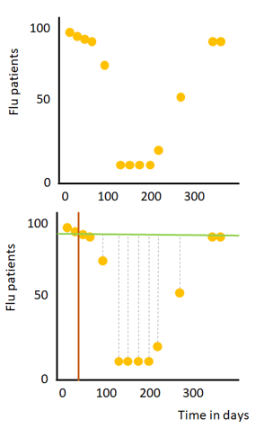
Let’s, for the sake of simplicity, imagine we have a data set with one numeric feature (the day in a year, i.e. January 1st, is day 1) and a numerical target variable (the number of flu patients in a hospital), see the image on the right. First, we have to identify which split should be used for the root-node. This process can be broken down in a few (iterative) steps:
1) Draw a line between two consecutive points to split the data into two subsets (orange line).
2) Calculate the mean amount of flu patients for these two points and draw a horizontal line through this calculated mean (green line)
3) Calculate the mean squared error (grey dashed lines) for all data points of the two created subsets
4) Repeat step 1 to 3, for every possible line between two consecutive points.
The split with the lowest MSE is selected in the root-node. This root-node splits the data into two subsets and the process is repeated for both created subsets. Note: in real-world datasets with multiple features the MSE for all possible splits for all features in the dataset are calculated and the split with the lowest MSE is selected in the node. This process can be repeated until all points are in a separate leaf which will provide perfect predictions for your training data, but not so accurate for new (test-)data (in other words; the model is overfitting). Overfitting is often avoided by for example setting a minimum number of samples that is required for a split. If multiple observations end up in a leaf, the predicted value is the mean value of all observations in the leaf (in our example the mean flu patients of all observations in the leaf).
The accuracy of a model is a trade-off between bias and variance. Trees are easy to build, interpret and use however ‘trees have one aspect that prevents them from being the ideal tool for predictive learning, namely inaccuracy’[2]. Trees can accurately classify the training data set, but do not generalize well to new datasets. In the next sections I will discuss two algorithms which are based on decision trees and use different approaches to enhance the accuracy of a decision tree: Random forests which is based on bagging and Gradient boosting that as the name suggests uses a technique called boosting. Bagging and boosting are both ensemble techniques, which basically means that both approaches combine multiple weak learners to create a model with a lower error than individual learners. The most obvious difference between the two approaches is that bagging builds all weak learners simultaneously and independently, whereas boosting builds the models subsequently and uses the information of the previously built ones to improve the accuracy.
Note: bagging and boosting can use several algorithms as base algorithms and are thus not limited to using decision trees.
As mentioned before a Random forest is a bagging (or bootstrap aggregating) method that builds decision trees simultaneously. Subsequently, it combines the predictions of the individual grown trees to provide a final prediction. A Random forest can be used for both regression and classification problems.
First, the desired number of trees have to be determined. All those trees are grown simultaneously. To prevent the trees from being identical, two methods are used.
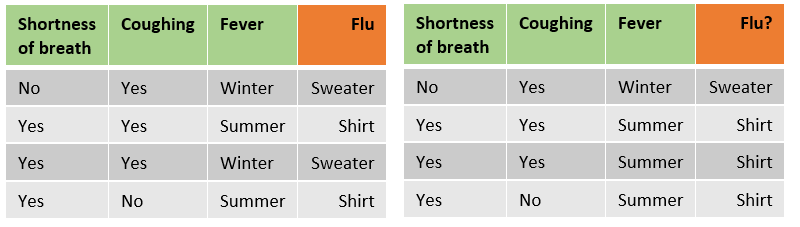
Step 1: First, for each tree a bootstrapped data set is created. This means that samples (rows) from the original data are randomly picked for the bootstrapped data set. The samples can be selected multiple times for a single bootstrapped data set (see below image).
 Original dataset on the left and bootstrapped dataset on the right
Step 2: For each bootstrapped data set a decision tree is grown. But for each step in the building process only a (predefined number of) randomly selected features (in our example 2) is used (often the square root of the number of features). For example, to define which feature should be in the root-node, we randomly select 2 features, calculate the impurity of these features and select the features with the least impurity. For the next step, we randomly select 2 other features (in our example, after selecting the root-node only 2 features are left, but in larger datasets you will select 2 new features at each step). Similar to building a single decision tree, the trees are grown until impurity does not improve anymore (or until a predefined max depth). In Random forests building deep trees does not automatically imply overfitting, due to the fact that the ultimate prediction is based on the mean prediction (or majority vote) of all combined trees. Several techniques can be used to tune a Random forest (for example the minimum impurity decrease or a minimum number of samples that have to be in a leaf), but I will not discuss the effects of these methods in this blog.
As a result of the bootstrapping and random feature selection, the different trees will have different architectures.
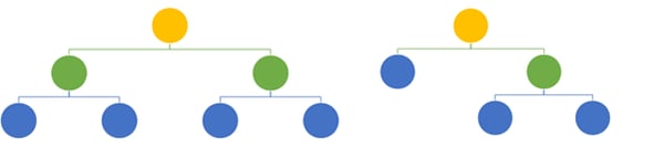
Two trees with different architectures built with a random forest algorithm
The Random forest can now be used to make predictions of new examples. The predictions of all individual trees in the random forests are combined and (in case of a classification problem) the class with the most predictions is the final prediction.
Gradient boosting is one of the most popular machine learning algorithms. Although it is easy to implement out-of-the-box by using libraries such as scikit-learn, understanding the mathematical details can ease the process of tuning the algorithm and eventually lead to better results. The main idea of boosting is to build weak predictors subsequently and use information of the previous built predictors to enhance performance of the model. For Gradient boosting these predictors are decision trees. In comparison to Random forest, the depth of the decision trees that are used is often a lot smaller in Gradient boosting. The standard tree-depth in the scikit-learn RandomForestRegressor is not set, while in the GradientBoostingRegressor trees are standard pruned at a depth of 3. This is important because individual trees can easily overfit the data, and while Random forest tackles this problem by averaging the prediction of all individual trees, Gradient boosting builds upon the results of the previous built tree. Therefore, individual overfitted trees can have large effect in Gradient Boosting. As a result of the small depth, individual trees built during Gradient boosting will thus probably have a larger bias.
In the next section, I will provide a mathematical deep dive on using gradient boost for a regression problem, but it can be used for classification as well. Gradient boosting for classification will not be covered in this blog, however the intuition has a lot in common with gradient boosting for regression. If you want to dive deeper into gradient boost for classification, I recommend you to watch the excellent videos of StatQuest (https://www.youtube.com/watch?v=jxuNLH5dXCs).
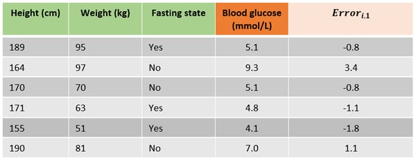
Let’s have a look at an example in which we want to predict a patient’s blood glucose using the height, weight and if the patient is in a fasting state state.
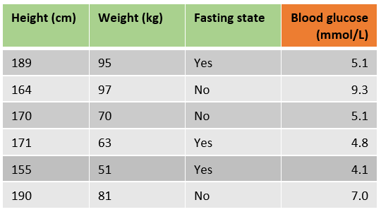
Gradient boosting uses a loss function to optimize the algorithm, the standard loss function for one observation in the scikit-learn implementation is least squares: 1/2 * (observed-predicted)²
The process of fitting a gradient boost regressor can be divided into several steps.
Step 1. The first step in Gradient boosting for regression is making an initial prediction by using the formula
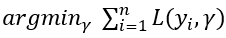
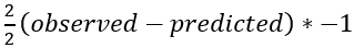
In other words, find the value of γ for which the sum of the squared error is the lowest. This can be solved by gradient descent to find where the derivative of the formula equals 0. By using the chain rule we know the derivative of
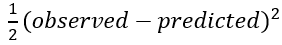
is equal to
For our sample data that would mean that we can find the best initial prediction by solving -(5.1-predicted)+-(9.3-predicted)+⋯+ -(7.0-predicted)=0. This yields 6*predicted=35.4 and therefore the best initial prediction is 35.4/6=5.9 mmol/L. Note that this is just the average of the target variable column.
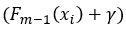
Step 2. As mentioned before, Gradient boosting uses previous built learners to further optimize the algorithm. Therefore, the trees in Gradient boosting are not fit on the target variable, but on the error or difference between predicted and observed values. The next step is to calculate the error for each sample by using the following formula:
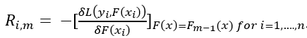
where m is the current tree (remember we are building a predefined number of trees subsequently) and n is the number of samples. This looks challenging, but really isn’t. The first part
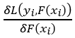
which is the derivative of the loss function with respect to the predicted value. As we saw in step 1, using the chain rule this is just –(observed — predicted), the big minus sign in front of the initial equation lets us end up with the observed minus the predicted value.
The subscript
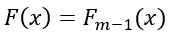
denotes that the values of the previous tree are used to predict the errors of the current tree. In short the error for a sample is the difference between the observed value and the predicted value in the previous tree.
In the following table the errors for all samples for building the first tree are added, which was just predicting the mean blood glucose for all samples.
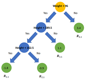
Step 3. The next step is to fit a decision tree with a predefined max depth on the errors instead of the target variable. By pruning the tree (or i.e. setting the maximum number of leaves) some leaves will end up with multiple errors. On the right is a tree fitted on the errors. The leaves are denoted with Rj,m where j is the leaf number and m the current tree. As the example data set is very small the leaves R(1,1), R(3,1) & R(4,1) all only include one sample. R(2,1) includes three samples with errors -1.1, -0.8 and -0.8.
Step 4. Determine the output value for each leaf. This can be done with a similar formula we used in step 1,

The major difference is that we are calculating a best prediction γ for each leaf j in tree m, instead of prediction one value for the entire data set. In addition, in order to calculate the best value to predict for a certain leaf, only the samples in that leaf are taken into account:

The last difference is that the predictions of the previous tree are used with an additional term γ:
Resulting from the choice in loss function, each leaf’s best value to predict is the average of the errors in this leaf. For leaf R(2,1) the best predicted value is -0.9 (the average of the errors [-1.1, -0.8, -0.8]).
Step 5. Make new predictions for all samples using the initial predictions and all built trees, using
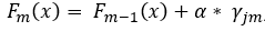
, where
d![]()
is the prediction of the sample’s leaf in the current tree and α is a predefined learning rate. Setting a learning rate reduces the effect of a single tree on the final prediction and improves accuracy. Simply speaking, the previous prediction for a sample is updated with the new predicted error from the current built tree. To illustrate this, we will predict first sample using the initial prediction and the first built tree with a learning rate of 0.1. In our newly built tree, this sample will end up in the second leaf with a prediction of -0.9.

. Although the difference with the initial prediction is small, the new prediction is closer to the observed blood glucose.
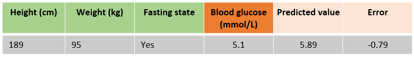
One sample including the predicted value and error after building the second tree
Step 6. Repeat step 2, 3 and 4 until the desired number of trees are built or adding new trees does not improve the fit. The result is a Gradient boosting model 😊.
This blog provides an overview of the basic intuition behind decision trees, Random forests and Gradient boosting. Hopefully this will provide you with a strong understanding if you implement these algorithms with libraries as scikit-learn and help you tuning the parameters of your model in the future and obtaining higher accuracy in the long run.
Special thanks to Mike Kraus and Loek Gerrits
[1] Theoretical comparison between the Gini Index and Information Gain criteria. Laura Elena Raileanu and Kilian Stoffel. https://www.unine.ch/files/live/sites/imi/files/shared/documents/papers/Gini_index_fulltext.pdf
[2] The Elements of Statistical Learning: Data Mining, Inference, and Prediction. Trevor Hastie, Robert Tibshirani and Jerome Friedman.