
Spoiler alert: you should use SHAP to understand your complex machine learning algorithm.
In some projects, finding the features that are crucial for a model, and describing how they impact the model, can be just as important as the performance of the model itself. For example, consider the following case:
A company’s KPI is reported via a number. The company is interested in finding the features that affect the value of the KPI, and they hire a data scientist for this task. The data scientist that they hire decides to do ML model that predicts the value of the KPI from a set of features (input variables), and the performance of this model is satisfactory. How can we learn from this model, in order to tackle the goal of the company? How can we tell which features are the most influential for the KPI? And how exactly are they influential?
The problem of feature importance is particularly relevant nowadays, when the algorithms used to solve problems can be extremely complex, and knowing the parameters that describe the model does not translate to an intuitive understanding of the workings of the algorithm. With simple models, such as linear regression, the impacts of a features are clear from the parameters. But this is not the case for more complex models, and it will never be: a feature may not have a single contribution on the model, but rather the contribution it has on the outcome depends on the combination of the values of all the features.
Imagine you are solving binary classification problem. The model is working wonderfully, since the predictions are accurate.
However to obtain such good results, you have to use an ensemble model, namely, a Random Forest Classifier. How can we figure out the inner workings of this model?
We can figure this out by calculating the Shapley values. Shapley values express the contribution that features have on the output of a model. This post focuses on providing the elements needed to understand, interpret and construct Shapley values in the context of supervised machine learning projects. Here we go:
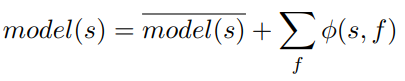
From the formula we can see that the Shapley values give the degree at which the features contribute to the value model(s).
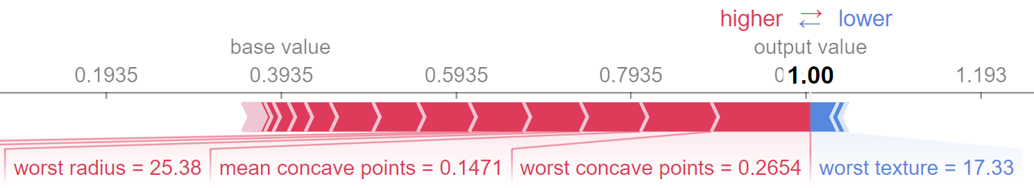
The Shapley values of a single sample s can be shown via a force plot shown below. This plot gives an idea of the contribution of features. In the plot, we observe that the base value is .3935
The output value of our model for this sample is 1, and the forceplot shows the positive Shapley values ϕ(s,f) in red and the negative ones in blue. The features worst concave points, mean concave points and worst radius contributed to an increase in the value of the predictions, while worst texture contributed to a decrease.
The real question is, of course, how to calculate the values ϕ(s,f)? The formula, as the Shapley values, come from Game Theory, and you can find it here, as well as the mathematical properties of Shapley values. It can take some time to understand the concepts on which the formula is based, and the motivations for it, but it is intuitively sound. Here we highlight two crucial considerations in the context of machine learning:
SHAP brings Shapley values from the computationally expensive to the practical realm. SHAP is a method to estimate Shapley values, which has its own python package that provides a set of visualizations to describe them (like the plot above). With this tool we are able to disclose the feature importance of the model. The mathematics behind these methods can be summarized as:
In this plot, the features are ordered top to bottom by how large their contributions are, so that the most influential feature for our model is worst concave points. At each feature f, the plot shows the distribution of Shapley values ϕ(s,f) for all s in the training set (since we are using a tree-based model, SHAP and Shapley values are the same). The value that each sample has at the specific feature is represented with the color.
Therefore, from the plot we can see that large values of worst concave points typically contribute to the probability of belonging to class 1 by around .1 and in some cases up to .2. We say typically because, as we have emphasized, the impact of the value of the feature depends on the whole sample, which is why we still have some red dots on the left side of worst concave points. Depending on the project, these cases may be interesting to look into further.
Remember from the force plot that the base value for our model is .3935. So that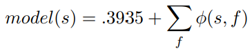
If a high value of worst concave points usually makes a sample to have an output value increase of .1 or .2 then for a sample that has a high value of worst concave point the expected output value would typically increase from .3935 to around .55 (if no extra information is given about the values of the other features).
So that’s how you can interpret the plots above and understand better your algorithm. I would like to add the following two warnings for interpretation:
So remember, the next time you want to describe how your algorithm works, be sharp about it. Be SHAP.
The code can be found here